Lesson 13: Model Build, Train, Evaluate

Next, we split the data into training (80%) and testing (20%).

main.py

# ...
 
from sklearn.model_selection import train_test_split
 
# ...
 
print(x[0:5])
 
x_train,x_test,y_train,y_test = train_test_split(x,y,test_size=0.2,random_state=0)
 
print(x_train.shape)
# Result: (414, 2)

Next, we import the linear regression and build/train the model:

main.py

# ...
from sklearn.linear_model import LinearRegression
 
# ...
 
print(x_train.shape)
 
model = LinearRegression()
model.fit(x_train, y_train)

Finally, we try to make the predictions of salaries for testing data based on the model trained on the training data:

main.py

# ...
 
model.fit(x_train, y_train)
 
y_pred = model.predict(x_test)
print(y_pred)

main.py

# Result:
([1199.71172545, 3090.85570562, 1199.71172545, 2446.32022189,
       1199.71172545, 3191.20120774, 2245.62921766, 1199.71172545,
       2647.01122613, 2245.62921766, 2044.93821342, 1300.05722757,
       3592.58321622, 3191.20120774, 2145.28371554, 1199.71172545,
       2647.01122613, 3291.54670986, 3191.20120774, 2044.93821342,
       3391.89221198, 2044.93821342, 3191.20120774, 3090.85570562,
       1199.71172545, 3090.85570562, 3592.58321622, 1199.71172545,
       2245.62921766, 3592.58321622, 2145.28371554, 2145.28371554,
       3391.89221198, 1199.71172545, 3592.58321622, 2145.28371554,
       2145.28371554, 2245.62921766, 3592.58321622, 1400.40272969,
       2145.28371554, 2145.28371554, 3391.89221198, 3592.58321622,
       1944.5927113 , 2847.70223037, 1300.05722757, 1199.71172545,
       1199.71172545, 3492.2377141 , 1300.05722757, 1944.5927113 ,
       1300.05722757, 2446.32022189, 2245.62921766, 3592.58321622,
       1300.05722757, 2446.32022189, 2145.28371554, 1300.05722757,
       2145.28371554, 3592.58321622, 3592.58321622, 1199.71172545,
       1500.74823181, 1944.5927113 , 2245.62921766, 2446.32022189,
       1300.05722757, 2446.32022189, 3391.89221198, 3191.20120774,
       2546.66572401, 2345.97471978, 2044.93821342, 3391.89221198,
       2245.62921766, 2145.28371554, 2044.93821342, 3592.58321622,
       2890.16470138, 2345.97471978, 2145.28371554, 3592.58321622,
       2847.70223037, 3391.89221198, 2345.97471978, 2245.62921766,
       3492.2377141 , 2446.32022189, 2145.28371554, 2847.70223037,
       3592.58321622, 2345.97471978, 3592.58321622, 2345.97471978,
       2345.97471978, 3291.54670986, 2245.62921766, 2044.93821342,
       3291.54670986, 3492.2377141 , 2245.62921766, 2245.62921766])

Ok, so we have 104 predictions. Are they accurate?

main.py

# ...
 
print(y_pred)
 
salaries = model.predict([[3, 12], [1, 1]])
print(salaries)

main.py

# Result:
([3793.27422045, 1199.71172545])

So, the model predicts a salary of 3793 Eur for 12 years of experience and 1199 Eur for 1 year of experience. Sounds similar to the reality. But how do we evaluate the accuracy?

For that, we try to see the R2 score:

main.py

# ...
from sklearn.metrics import r2_score
 
# ...
 
print(salaries)
 
r2 = r2_score(y_test, y_pred)
 
print(f"R2 Score: {r2} ({r2:.2%})")

main.py

# Result:
R2 Score: 0.6311227637903979 (63.11%)

Hmmmm... 63.11% is our "final result". Such accuracy of the model is not that great, is it?

But this is actually the overall point I want to make with this example. Real-life data is messy. It may be inaccurate. It may be hard to predict the results.

Looking from another angle, 63% isn't THAT bad. It may be acceptable in some cases, depending on the project's goals. It's bigger than 50%, so it's something!

What If We Did It Without Filters?

I also promised to show you what the predictions would be if we made them without filtering out the outliers of 6000+ Eur salaries.

So, we would just skip this ONE line:

main.py

# ...
 
df = df[df['salary'] <= 6000]
 
# ...

I tried to do it, and here's the result.

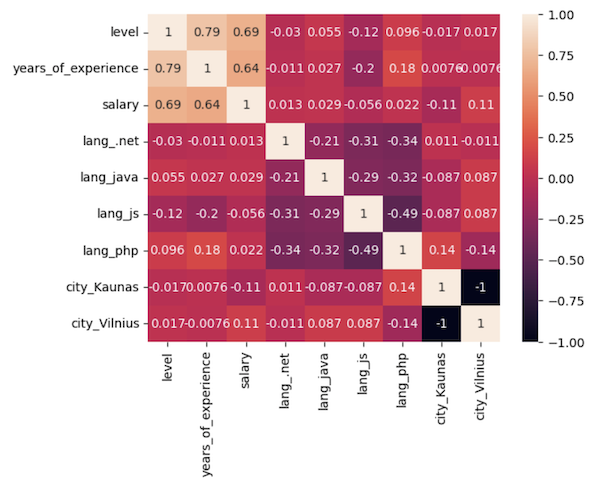
Visual correlation heatmap shows lower numbers:

And the overall R2 score is also lower:

R2 Score: 0.5305925405861269 (53.06%)

So, the accuracy is 10% lower. This proves that data pre-processing is VERY important, as it may affect the model's accuracy significantly.

Final File

If you felt lost in the code above, here's the final file with all the code from this lesson:

main.py

import pandas as pd
import numpy as np
import matplotlib.pyplot as plt
import seaborn as sns
from sklearn.model_selection import train_test_split
from sklearn.linear_model import LinearRegression
from sklearn.metrics import r2_score
 
df = pd.read_csv('salaries-2023.csv')
 
print(df.head())
print(df.shape)
df.info()
print(df.describe())
 
allowed_languages = ['php', 'js', '.net', 'java']
df = df[df['language'].isin(allowed_languages)]
 
vilnius_names = ['Vilniuj', 'Vilniua', 'VILNIUJE', 'VILNIUS', 'vilnius', 'Vilniuje']
condition = df['city'].isin(vilnius_names)
df.loc[condition, 'city'] = 'Vilnius'
 
kaunas_names = ['KAUNAS', 'kaunas', 'Kaune']
condition = df['city'].isin(kaunas_names)
df.loc[condition, 'city'] = 'Kaunas'
 
print(df.city.value_counts())
 
allowed_cities = ['Vilnius', 'Kaunas']
df = df[df['city'].isin(allowed_cities)]
print(df.shape)
 
df_sorted = df.sort_values(by='salary', ascending=False)
print(df_sorted.head(20))
 
x = df.iloc[:, -2:-1]
y = df.iloc[:, -1].values
plt.xlabel('Years of experience')
plt.ylabel('Salary')
plt.scatter(x, y)
plt.show()
 
df = df[df['salary'] <= 6000]
print(df.shape)
 
x = df.iloc[:, -2:-1]
y = df.iloc[:, -1].values
plt.xlabel('Years of experience')
plt.ylabel('Salary')
plt.scatter(x, y)
plt.show()
 
one_hot = pd.get_dummies(df['language'], prefix='lang')
df = df.join(one_hot)
df = df.drop('language', axis=1)
 
one_hot = pd.get_dummies(df['city'], prefix='city')
df = df.join(one_hot)
df = df.drop('city', axis=1)
 
print(df.head(10))
 
sns.heatmap(df.corr(), annot=True)
plt.show()
 
x = df.iloc[:, 0:2].values  # we take only years and level
y = df.iloc[:, 2].values  # we take the salary
print(x[0:5])
 
print(y[0:5])
 
x_train, x_test, y_train, y_test = train_test_split(x, y, test_size=0.2, random_state=0)
print(x_train.shape)
 
model = LinearRegression()
model.fit(x_train, y_train)
 
y_pred = model.predict(x_test)
print(y_pred)
 
salaries = model.predict([[3, 12], [1, 1]])
print(salaries)
 
r2 = r2_score(y_test, y_pred)
 
print(f"R2 Score: {r2} ({r2:.2%})")

This is the end of this tutorial about real-life scenarios with salaries.

The main goal here was to show you the importance of preparing the data for the ML models so they would be more accurate.

What's next? You may read how to make your Machine Learning model available for public, by deploying it on remote server. Here's our tutorial: Publish ML Model as API or Web Page: Flask and Digital Ocean