Lesson 5: Model Training, Prediction, Evaluation

So now, as we have our data split, we can train the model based on the Linear Regression algorithm.

Step 1. Model Training and Prediction

We will create the linear regressor model using the scikit-learn library: developers often call that variable model or regressor.

main.py

import pandas as pd
import numpy as np
import matplotlib.pyplot as plt
from sklearn.model_selection import train_test_split
from sklearn.linear_model import LinearRegression
 
df = pd.read_csv("salaries.csv")
 
x = df.iloc[:,:-1].values  # get all rows with all columns except the last one
y = df.iloc[:,-1].values   # get all rows with only the last column
 
x_train,x_test,y_train,y_test = train_test_split(x,y,test_size=0.2,random_state=0)
 
model = LinearRegression()
 
plt.scatter(x, y)
plt.show()

At this moment, our model doesn't really do anything yet, so we need to "tell it what to do". We train it with the data, using the .fit() method and passing our training data.

main.py

# ...
 
model = LinearRegression()
model.fit(x_train, y_train)
 
# ...

Now, as our model knows about the initial training data, we can ask it to predict the values of the data in the testing split.

We pass the x_test and see what it would predict for y values. The resulted variable will be called y_pred, short for "predicted".

main.py

# ...
 
model.fit(x_train, y_train)
y_pred = model.predict(x_test)
print(y_pred)
 
# ...

main.py

# Result:
[2816.37966916 3779.68276414 3009.04028815 3779.68276414 3587.02214514
 2623.71905016 4165.00400213 3201.70090715 3587.02214514 3009.04028815
 2431.05843116 3587.02214514 3201.70090715 3587.02214514 3394.36152615
 3587.02214514 3779.68276414 2623.71905016 3201.70090715 2816.37966916]

As you can see, the predicted result is the array of 20 items, as we passed in the array of 20 values of years of experience.

We can also predict salaries for specific years of experience, which are not included in our initial data. That also includes fractions, like 2.5 years or 5.2 years of experience. Our model is already trained for it!

main.py

# ...
 
print(y_pred)
salaries = model.predict([[11], [13], [2.5], [5.2]])
print(salaries)
 
# ...

main.py

# Result:
[4357.66462113 4742.98585912 2720.04935966 3240.23303095]

So, the expected salary for 11 years of experience is 4357.66, and 13 years would predict a 4742.99 salary.

Notice that we pass the parameter as array of arrays (also called "matrix") because that's how our model was trained, the linear regression fit() and predict() methods accept the x parameter as a matrix, see the documentation.

Now, let's compare the predicted values with the actual values.

Step 2. Comparing Actual Test Data and Predicted Data

Our goal is to compare the items in the arrays of y_pred and y_test. First, let's try to do it just by listing them:

main.py

# ...
 
salaries = model.predict([[11], [13]])
print(salaries)
print(y_test)
 
# ...

main.py

# Result:
[2669 3661 2991 3751 3575 2672 4708 3070 3599 2884 2389 3397 3060 3281
 3269 3638 3638 2698 3099 2767]

So, we have the values like 2816.37 VS 2669, 3779.68 vs 3751. Close but not perfectly accurate. And it's not easy to compare those values jumping with eyes between two arrays, right? Luckily, we can just list the differences between the items.

main.py

# ...
 
print(y_test)
error = y_pred - y_test
print(error)
 
# ...

main.py

# Result:
[ 147.37966916  118.68276414   18.04028815   28.68276414   12.02214514
  -48.28094984 -542.99599787  131.70090715  -11.97785486  125.04028815
   42.05843116  190.02214514  141.70090715  306.02214514  125.36152615
  -50.97785486  141.68276414  -74.28094984  102.70090715   49.37966916]

We can also visualize it with matplotlib, showing both testing data dots and predicted results line on the same chart.

main.py

# ...
y_pred = model.predict(x_test)
 
error = y_pred - y_test
print(error)
 
plt.scatter(x_test, y_test)
plt.plot(x_test, y_pred, color="yellow")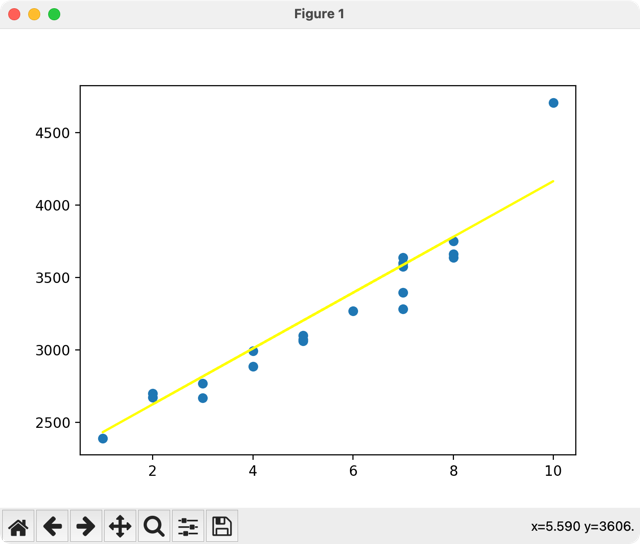
 
# ...

What conclusions can we draw from here?

The line of our prediction is pretty accurate, with only one dot being really far from the line. Such dots are called "noise", and we will discuss them in the future lessons.

That "noise" might have happened for various reasons, but usually, the main thing is the non-ideal initial data. We will talk about pre-processing later, but for now, we need to evaluate our model's training results in some kind of mathematical values: is it good for predictions or not?

Step 3. Evaluate Model Accuracy

To judge if our model's predictions are accurate, we need to choose the metrics for it. There are various options, but the most human-friendly to understand is the "R-squared score value" which comes from the scikit-learn library and varies from 0% to 100% accuracy.

main.py

import pandas as pd
import numpy as np
import matplotlib.pyplot as plt
from sklearn.model_selection import train_test_split
from sklearn.linear_model import LinearRegression
from sklearn.metrics import r2_score
 
df = pd.read_csv("salaries.csv")
 
x = df.iloc[:,:-1].values  # get all rows with all columns except the last one
y = df.iloc[:,-1].values   # get all rows with only the last column
 
x_train,x_test,y_train,y_test = train_test_split(x,y,test_size=0.2,random_state=0)
 
model = LinearRegression()
model.fit(x_train, y_train)
y_pred = model.predict(x_test)
 
r2 = r2_score(y_test, y_pred)
print(f"R2 Score: {r2} ({r2:.2%})")
 
plt.scatter(x_test, y_test)
plt.plot(x_test, y_pred, color="yellow")
plt.show()

main.py

# Result:
R2 Score: 0.8921287198195745 (89.21%)

That number of 0.8921 means 89.21% accuracy of our model predictions, which is considered pretty high. But, of course, the accuracy depends not only on the model algorithm but also on the initial data, so this is exactly what we will discuss in the next sections.

Notice: if you're unfamiliar with the Python f-string syntax for f"string" that we used above, here's the tutorial about it.

Also, there are other numbers from the same sklearn.metrics library that could help to evaluate the model, but we will talk about them in other tutorials or courses.

So yeah, we have our model for the first example!

But wait, isn't Machine Learning about mathematical formulas? And we haven't touched any math in this course, yet. So, in the next lesson, let's briefly cover that part.

Final File

If you felt lost in the code above, here's the final file with all the code from this lesson:

main.py

import pandas as pd
import numpy as np
import matplotlib.pyplot as plt
from sklearn.model_selection import train_test_split
from sklearn.linear_model import LinearRegression
from sklearn.metrics import r2_score
 
df = pd.read_csv("salaries.csv")
 
x = df.iloc[:,:-1].values  # get all rows with all columns except the last one
y = df.iloc[:,-1].values   # get all rows with only the last column
 
x_train,x_test,y_train,y_test = train_test_split(x,y,test_size=0.2,random_state=0)
 
model = LinearRegression()
model.fit(x_train, y_train)
y_pred = model.predict(x_test)
 
r2 = r2_score(y_test, y_pred)
print(f"R2 Score: {r2} ({r2:.2%})")
 
plt.scatter(x_test, y_test)
plt.plot(x_test, y_pred, color="yellow")
plt.show()