Importing Libraries and Reading Data

When working with machine learning projects, you will typically see these steps after you get the initial data:

Explore the data, looking at it from various angles
Preprocess/prepare the data for modeling
Choose the model/algorithms
Train the model
Evaluate the model

In previous lessons, we've seen points from 3 to 5, but in most real-life cases, points 1 and 2 are where you will spend most of your time as an ML engineer.

So our second mini-project is exactly what I want to showcase.

Task Description

So far, we looked at regression with pretty much an "ideal" data set: the equation was pretty linear, and the model's R2 score was around 90%.

That, unfortunately, rarely happens with data in real life. Real data is messy. That's why we almost always need to perform a set of steps before building the actual model:

Data exploration: looking at the data as an array in various shapes
Data cleaning: remove null values, deal with "noise" from outliers, change categories into numbers, etc.
Data visualization: trying to build graph(s) so we would understand which model to use

I want to show you an example based on real data - a survey of developers in my local community in Lithuania, asking them about their salaries in May of 2023.

After some initial cleanup for the purpose of this tutorial, the CSV with 760 answers looks like this:

You can view/download that CSV here. Also, you can check out the Jupyter Notebook for this example, here.

Our goal is to predict the salary by other independent variables:

Main programming language they work with (it was a free text input answer)
City they live in (in Lithuanian language) (free text input answer)
Level (dropdown: junior is 1, mid is 2, senior is 3)
Years of experience (dropdown: values 1 to 10)

But remember: this is SURVEY data. I don't have any proof that people actually answered accurately. So we need to check everything and "eliminate the noise".

Also, we don't even have a guarantee that salary can be accurately predicted by those parameters. Our goal is to TRY.

This is actually what your work will be as an ML engineer. You will often get "raw" unprepared data with some task to predict/classify the result. So, first, you would need to preprocess it even to begin modeling it.

So, let's dive in.

Importing Libraries and Reading Data

Let's start our Python script with the "already familiar stuff".

main.py

1import pandas as pd
2import numpy as np
3import matplotlib.pyplot as plt
4import seaborn as sns

The first three lines are familiar, and seaborn is a new library we haven't used yet. We will need it to build a correlation graph a bit later.

If you don't have it on your computer, install it with pip3 install seaborn.

main.py

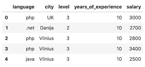
1# ...
2 
3import seaborn as sns
4 
5df = pd.read_csv('salaries-2023.csv')
6print(df.head())

The result will be the first 5 rows of the data set:

But if you take a closer look, we have NaN values in our data. Let's fix that with Pandas function dropna():

main.py

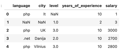
1# ...
2 
3df = pd.read_csv('salaries-2023.csv')
4df = df.dropna()
5print(df.head())

The result is the image you already saw above:

main.py

1# ...
2 
3print(df.head())
4 
5print(df.shape)
6# Result: (760, 5)

To explore the data in "overview" day, there are other useful pandas functions like info() and describe().

main.py

1# ...
2 
3print(df.shape)
4df.info()

Result:

 1RangeIndex: 760 entries, 0 to 759
 2Data columns (total 5 columns):
 3 #   Column               Non-Null Count  Dtype
 4---  ------               --------------  -----
 5 0   language             760 non-null    object
 6 1   city                 760 non-null    object
 7 2   level                760 non-null    int64
 8 3   years_of_experience  760 non-null    int64
 9 4   salary               760 non-null    int64
10dtypes: int64(3), object(2)
11memory usage: 29.8+ KB

This is primarily useful to find the null values and filter them out. But in this case, all 760 rows have non-null values.

main.py

1# ...
2 
3df.info()
4print(df.describe())

Result:

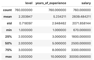
These terms are a bit harder to explain, but we have a separate article with more details: Pandas describe() Explained: Mean, Std, Percentiles

So now we have a general overview of what dataset we're dealing with. In the next lesson, we try to dig a bit deeper and decide what we can filter out.

Final File

If you felt lost in the code above, here's the final file with all the code from this lesson:

main.py

 1import pandas as pd
 2import numpy as np
 3import matplotlib.pyplot as plt
 4import seaborn as sns
 5 
 6df = pd.read_csv('salaries-2023.csv')
 7df = df.dropna()
 8 
 9print(df.head())
10print(df.shape)
11df.info()
12print(df.describe())