Lesson 7: Text Classification: Bigger CSV File and Other Algorithms

Now that we understand how Random Forest works for text classification, let's repeat the process for a more complex file: a 1226-line CSV file of IT products and multiple categories.

Notice: you can view/download that CSV here. Also, you can check out the Jupyter Notebook for this example, here.

We will also compare other algorithms against Random Forest in terms of accuracy.

Data Exploration

Let's read the CSV file and show what's inside.

# Importing the usual libraries
import pandas as pd
import numpy as np
from sklearn.feature_extraction.text import TfidfVectorizer
from sklearn.model_selection import train_test_split
 
from sklearn.ensemble import RandomForestClassifier
from sklearn.metrics import accuracy_score
 
df = pd.read_csv("devices-products.csv")
df.head()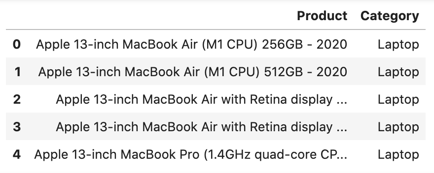

df.shape
 
# Result: (1226, 2)

Let's also see which categories are most popular:

df['Category'].value_counts()

Category
Laptop            452
Monitor           296
Desktop           259
Server             55
Smartphone         50
IoT                30
Tablet             22
Thin Client        16
Printer            11
Hard drive         11
Gaming              5
Workstation         4
Multimedia          4
Network             4
Entertainment       2
Converged Edge      2
Converged           2
SAN/NAS             1
Name: count, dtype: int64

Now, we have a general understanding of our data.

The task is still the same: predicting and auto-assigning the category for any new product by its name.

Vectors, Model Training and Predictions

Let's repeat the same code from the previous lesson - the only difference is the data we're working with:

x = df['Product'].values
y = df['Category'].values
 
x_train, x_test, y_train, y_test = train_test_split(x, y, test_size=0.2, random_state=0)
 
tfidf_vectorizer = TfidfVectorizer()
tfidf_train_vectors = tfidf_vectorizer.fit_transform(x_train)
tfidf_test_vectors = tfidf_vectorizer.transform(x_test)
 
clf_random_forest = RandomForestClassifier()
clf_random_forest.fit(tfidf_train_vectors, y_train)
y_pred = clf_random_forest.predict(tfidf_test_vectors)
 
df_compare = pd.DataFrame(
    data={
        'product': x_test,
        'predicted_category': y_pred,
        'real_category': y_test
    },
    columns=['product', 'predicted_category', 'real_category'])
df_compare

The full CSV file has 1226 rows, so the testing data is 20% of that. And for those 246 rows, we have these predictions:

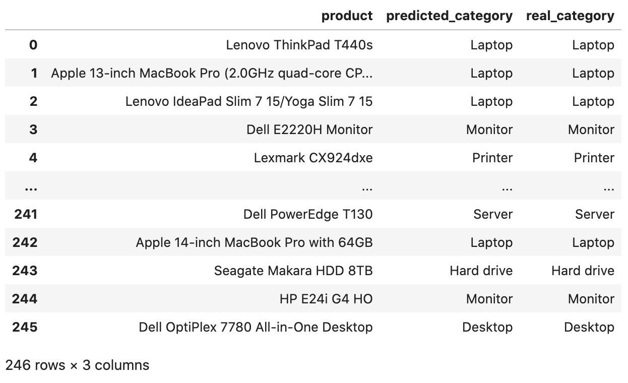
Those look all accurate, right?

But wait, we see only 10 lines here. What about the other values? Let's see the accuracy score:

accuracy_score(y_test, y_pred)
 
# Result: 0.9186991869918699

So, the accuracy is 91%, not 100%. In other words, it misclassified 20 products!

Is it acceptable or not? This question should be answered by the client who created that task in the first place. They should know the goals of the project. But generally, 90%+ accuracy is considered a good number.

Perhaps, in real life, this classification would be used only as a recommendation for the person who would enter new products via the web admin panel, so then the human interaction is needed to approve or decline the suggestion by the ML model.

Let's Briefly Touch Other Algorithms

We will dive deeper into other algorithms in other courses, but for now, you need to know their names at least and understand how to call them in Python.

As mentioned in the very first lesson of the course, we will talk about these most popular ones:

• Decision Trees and Random Forest (DONE)
• K-Nearest Neighbors (often shortened to KNN)
• Support Vector Machines (shortened to SVM)
• Logistic Regression
• Naive Bayes

Each of those algorithms has a function in the Python library scikit-learn, so our task as developers is just to call those functions with specific parameters and pass the data correctly.

I will just show you the code for training the model on each of those algorithms, and then we will compare the accuracy:

# Importing the usual libraries
import pandas as pd
import numpy as np
from sklearn.feature_extraction.text import TfidfVectorizer
from sklearn.model_selection import train_test_split
 
from sklearn.ensemble import RandomForestClassifier
from sklearn.metrics import accuracy_score
 
# Importing libraries for other algorithms
from sklearn.neighbors import KNeighborsClassifier
from sklearn.naive_bayes import MultinomialNB
from sklearn.svm import LinearSVC
from sklearn.linear_model import LogisticRegression
 
df = pd.read_csv("devices-products.csv")
x = df['Product'].values
y = df['Category'].values
 
x_train, x_test, y_train, y_test = train_test_split(x, y, test_size=0.2, random_state=0)
 
tfidf_vectorizer = TfidfVectorizer()
tfidf_train_vectors = tfidf_vectorizer.fit_transform(x_train)
tfidf_test_vectors = tfidf_vectorizer.transform(x_test)
 
clf_random_forest = RandomForestClassifier()
clf_random_forest.fit(tfidf_train_vectors, y_train)
y_random_forest_pred = clf_random_forest.predict(tfidf_test_vectors)
accuracy_score(y_test, y_random_forest_pred)
# Result: 0.9146341463414634
 
clf_knn = KNeighborsClassifier(n_neighbors=19)
clf_knn.fit(tfidf_train_vectors, y_train)
y_knn_pred = clf_knn.predict(tfidf_test_vectors)
accuracy_score(y_test, y_knn_pred)
# Result: 0.8577235772357723
 
clf_nb = MultinomialNB()
clf_nb.fit(tfidf_train_vectors, y_train)
y_nb_pred = clf_nb.predict(tfidf_test_vectors)
accuracy_score(y_test, y_nb_pred)
# Result: 0.8536585365853658
 
clf_svc = LinearSVC(dual=True)
clf_svc.fit(tfidf_train_vectors, y_train)
y_svc_pred = clf_svc.predict(tfidf_test_vectors)
accuracy_score(y_test, y_svc_pred)
# Result: 0.967479674796748
 
clf_logreg = LogisticRegression()
clf_logreg.fit(tfidf_train_vectors, y_train)
y_logreg_pred = clf_logreg.predict(tfidf_test_vectors)
accuracy_score(y_test, y_logreg_pred)
# Result: 0.9146341463414634

Accuracy results compared side-by-side:

{'random_forest': 0.9146341463414634,
 'k_nearest_neighbors': 0.8577235772357723,
 'naive_baynes': 0.8536585365853658,
 'support_vector_machines': 0.967479674796748,
 'logistic_regression': 0.9146341463414634}

As you can see, you can get significantly different accuracy with different algorithms: from 85.3% to 96.7%!

Compare Algorithm Speed Performance

In this simple case, with only ~1k records, all algorithms will be relatively quick to execute. However, we can still measure the exact timings to understand the relative differences between the algorithms.

For better visualization, let's create two sets: scores and times, then show their data at the end.

To measure the time, I will add a library timeit and a start point before creating each classifier.

The full code:

# In the beginning - import and default values
import timeit
 
scores = {}
times = {}
 
# ...
# Then, each algorithm will start with `start`
#   and end with assigning the `score` and `times`
 
start = timeit.default_timer() 
clf_random_forest = RandomForestClassifier()
clf_random_forest.fit(tfidf_train_vectors, y_train)
y_random_forest_pred = clf_random_forest.predict(tfidf_test_vectors)
scores['random_forest'] = accuracy_score(y_test, y_random_forest_pred) 
times['random_forest'] = timeit.default_timer() - start 
 
start = timeit.default_timer() 
clf_knn = KNeighborsClassifier(n_neighbors=19)
clf_knn.fit(tfidf_train_vectors, y_train)
y_knn_pred = clf_knn.predict(tfidf_test_vectors)
scores['k_nearest_neighbors'] = accuracy_score(y_test, y_knn_pred) 
times['k_nearest_neighbors'] = timeit.default_timer() - start 
 
start = timeit.default_timer() 
clf_nb = MultinomialNB()
clf_nb.fit(tfidf_train_vectors, y_train)
y_nb_pred = clf_nb.predict(tfidf_test_vectors)
scores['naive_baynes'] = accuracy_score(y_test, y_nb_pred) 
times['naive_baynes'] = timeit.default_timer() - start 
 
start = timeit.default_timer() 
clf_svc = LinearSVC(dual=True)
clf_svc.fit(tfidf_train_vectors, y_train)
y_svc_pred = clf_svc.predict(tfidf_test_vectors)
scores['support_vector_machines'] = accuracy_score(y_test, y_svc_pred) 
times['support_vector_machines'] = timeit.default_timer() - start 
 
start = timeit.default_timer() 
clf_logreg = LogisticRegression()
clf_logreg.fit(tfidf_train_vectors, y_train)
y_logreg_pred = clf_logreg.predict(tfidf_test_vectors)
scores['logistic_regression'] = accuracy_score(y_test, y_logreg_pred) 
times['logistic_regression'] = timeit.default_timer() - start 

Then, at the end of the script, we create a list of all the algorithms and iterate through them, showing scores and times:

algorithms = [
    'random_forest',
    'k_nearest_neighbors',
    'naive_baynes',
    'support_vector_machines',
    'logistic_regression'
]
 
for i in range(5):
    print(f"{algorithms[i]}: {scores[algorithms[i]]:.2%} ({times[algorithms[i]]:.2}s)")

# Result:
random_forest: 91.06% (0.3s)
k_nearest_neighbors: 85.77% (0.022s)
naive_baynes: 85.37% (0.0074s)
support_vector_machines: 96.75% (0.021s)
logistic_regression: 91.46% (0.17s)

As I mentioned above, Random Forest is accurate but slower, and from other algorithms, Support Vector Machines show the best accuracy with great speed. So, possibly, that algorithm would make the most sense for this dataset.

That's why the job of the ML engineer is to "sense" which algorithm would perform the best in which scenario and test multiple algorithms with their parameters before deploying the ML model to run predictions on "live" data.

As I mentioned, we'll not be touching other algorithms deeper in this course. For now, I just wanted to quickly show their "overview" so you would have a general understanding of what's available on the market.

What's next? You may read how to make your Machine Learning model available for the public, by deploying it on a remote server. Here's our tutorial: Publish ML Model as API or Web Page: Flask and Digital Ocean