Split Data and Train/Build the Model

In the previous lesson, we analyzed our data. Now, we will build the model and predict the tweet virality.

Split into Features/Target with `iloc[]`

In classification problems, we have two parts of the data:

All the columns that are the information/input: those will go to the x variable, often called "feature(s)"
One column which value we need to predict: this will go to the y variable, often called "target"

For that split, we will use the iloc syntax of the dataframe:

x = df.iloc[:,:-1].values
y = df.iloc[:,-1].values

This syntax is complex to understand if you haven't seen it before.

The general syntax of iloc[] is this: df.iloc[row(s), column(s)].

Both rows and columns can be defined in such ways:

One single column like "0" (the first column) or "-1" (meaning the first column from the end)
Or as a range of columns with a ":" separator, like "1:3" would mean rows/columns from 1 to 3. The syntax ":" means all rows/columns.

So, now look at our examples above again.

For the x variable, we're taking all the rows and all the columns except the last one.

For the y variable, we're also taking all the rows, but now only the last column.

These will be the values of the first five rows:

x[0:5]

# Result:
array([[ 10,   2,   0],
       [123,  14,   5],
       [203,  34,  29],
       [ 23,   2,   3],
       [  1,   0,   0]])

y[0:5]

# Result:
array([0, 1, 1, 0, 0])

Split into Training/Testing

As I mentioned before, our model will be trained on a subset of the existing data. And then, we will use the remaining subset to test if the model has correct predictions.

To split the data, we will use the scikit-learn function called train_test_split():

x_train, x_test, y_train, y_test = train_test_split(x, y, test_size=0.2, random_state=0)

The parameter test_size=0.2 means we allocate 20% of the data for testing and 80% for training.

The parameter random_state is important but from the angle of whether its value exists or not. You can read more in this tutorial: Method train_test_split(): Best Value for random_state Parameter?

As a result, we will have four data structures:

x_train and y_train for training
x_test and y_test for testing

x_train.shape
 
# Result: (80, 3)

Build and Train The Model

This is probably the most important part of ML script: choosing the algorithm and passing the data to it:

clf = RandomForestClassifier()
clf.fit(x_train, y_train)

The variable name clf is short for "classifier". By this time, you already may have noticed how Python ML engineers like to shorten the variable names.

We had imported that RandomForestClassifier() earlier on top with the code from sklearn.ensemble import RandomForestClassifier.

At this point, we don't have any visual results, but our model has been trained using 80% of our data. In other words, it has learned what tweets are viral or not, depending on the engagement numbers.

Model Predictions

Now, it's time to test if our model would predict the correct results. We will use the function clf.predict() for that.

First, we can do it manually.

Let's pass the data for two random tweets and see the result:

A tweet with 5 likes, 5 retweets and 5 replies
A tweet with 199 likes, 20 retweets and 1 reply

We put those into a list and pass to the classifier model:

viral_predict = clf.predict([[5, 5, 5], [199, 20, 1]])
viral_predict
 
# Result: array([0, 1])

As you can see, the first tweet with the 5/5/5 combination was marked as 0 (not viral), and the second one with 199/20/1 was classified as viral. That sounds about correct!

But, of course, we can't trust the model's accuracy from just a few manual examples. That's what we have our testing data for. Remember x_test and y_test?

So, let's pass the x_test to our model and compare that with the y_test values.

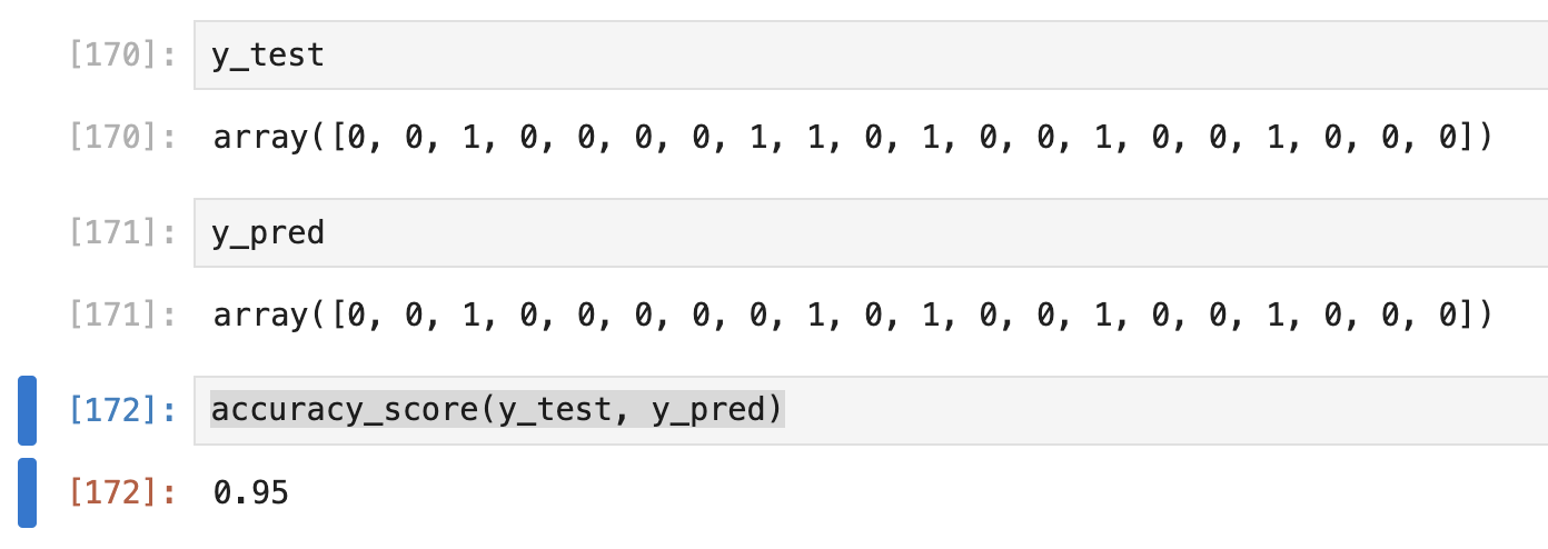
y_pred = clf.predict(x_test)
y_pred
 
# Result: 20 items predicted
array([0, 0, 1, 0, 0, 0, 0, 0, 0, 0, 0, 0, 0, 0, 0, 1, 0, 1, 0, 1])

Let's compare that to the y_test:

y_test
 
# Result: from the testing data
array([0, 0, 1, 0, 0, 0, 0, 0, 0, 0, 0, 0, 0, 0, 0, 1, 0, 1, 0, 1])

Not clear enough? Let's compare in a table:

df_compare = pd.DataFrame(
    data={
        'likes': x_test[:,0],
        'retweets': x_test[:,1],
        'replies': x_test[:,2],
        'predicted_value': y_pred,
        'real_value': y_test
    },
    columns=['likes', 'retweets', 'replies', 'predicted_value', 'real_value'])
df_compare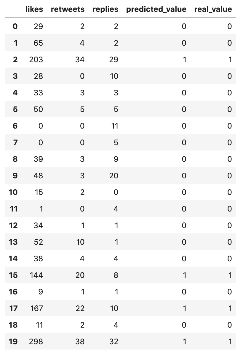

The last two column values look identical to me. So, our model has made 100% accurate predictions!

Just to make sure, let's officially test the accuracy with the automatic calculations.

Model Accuracy and Project Conclusions

To test the accuracy, we will use the function accuracy_score():

accuracy_score(y_test, y_pred)
 
# Result: 1.0

Yay, we have 1.0, which means 100%!

I've also tried to train the model without the random_state parameter, which means totally randomizing train/test data every time, and the accuracy fluctuated a bit between 95-100%:

It is still a great result!

But I admit, this example is overly simplistic, with only 100 rows of data. Unfortunately, with more real-world data, the accuracy of 95-100% is rarely seen.

For real-world applications, the clients are usually happy with 90% accuracy, and even that is hard to achieve. We will show that in other examples of this course.

The goal for this example was to show you the process of how we read the data, split it, and then train/evaluate the model.

The Full Code

You can check out the Jupyter Notebook for this whole project here.

Or, if you prefer IDE like PyCharm, you can copy-paste this code into there:

import pandas as pd
import numpy as np
from sklearn.model_selection import train_test_split
from sklearn.ensemble import RandomForestClassifier
from sklearn.metrics import accuracy_score
 
df = pd.read_csv("tweets.csv")
print(df.head())
 
print(df.shape)
 
print(df['is_viral'].value_counts())
 
x = df.iloc[:,:-1].values
y = df.iloc[:,-1].values
 
x_train, x_test, y_train, y_test = train_test_split(x, y, test_size=0.2, random_state=0)
 
clf = RandomForestClassifier()
clf.fit(x_train, y_train)
 
viral_predict = clf.predict([[5, 5, 5], [199, 20, 1]])
print(viral_predict)
 
y_pred = clf.predict(x_test)
 
df_compare = pd.DataFrame(
    data={
        'likes': x_test[:,0],
        'retweets': x_test[:,1],
        'replies': x_test[:,2],
        'predicted_value': y_pred,
        'real_value': y_test
    },
    columns=['likes', 'retweets', 'replies', 'predicted_value', 'real_value'])
print(df_compare)
 
print(accuracy_score(y_test, y_pred))

In the next lesson, we will repeat this process with more complex data, also explaining the algorithm theory along the way.

Split into Features/Target with iloc[]