Classification Example with Multiple Categories

In the last lesson, we tried to predict whether the tweet is viral, which is a binary classification. Now, what if we have more than two categories?

Let's try to run the same script with the same Random Forest classification algorithm (yes, I'm still yet to explain how it works under the hood, in the next lesson) and see if it performs the same way.

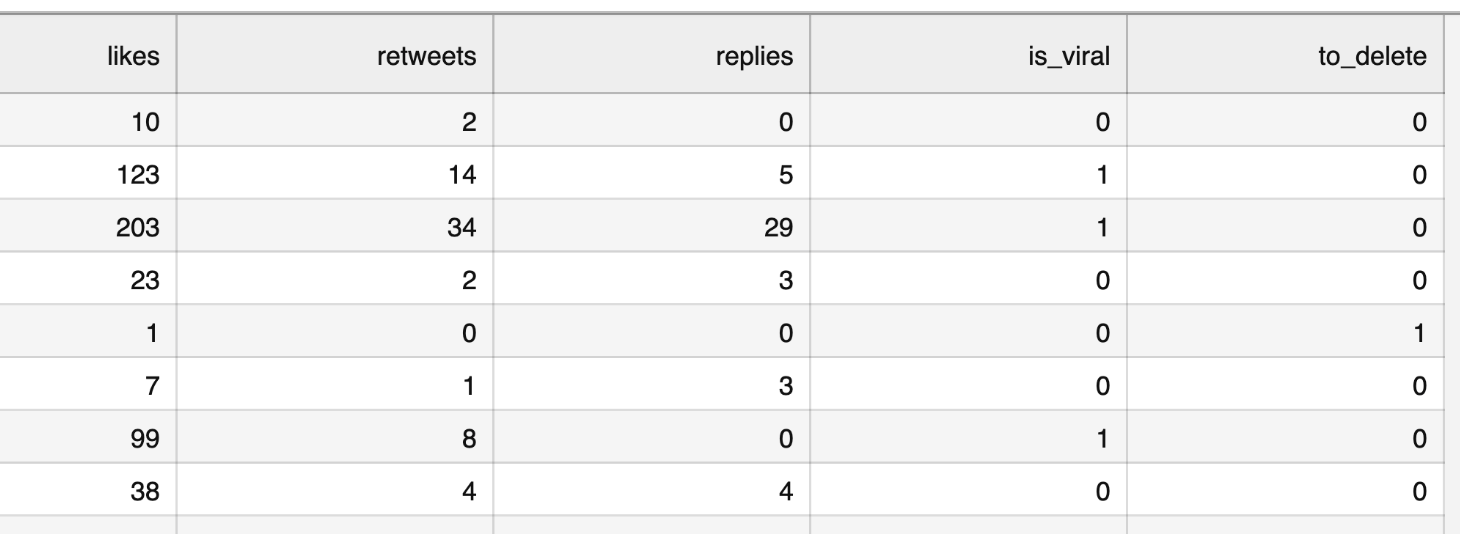
In addition to is_viral, let's add another option of to_delete, which means that the tweet performed so poorly that it's worth deleting it from your profile.

So, here's our updated CSV file:

Notice: you can view/download that CSV here. Also, you can check out the Jupyter Notebook for this example, here.

Again, first, there's a human effort to classify the first 100 tweets, and then the ML model should take over the task.

In fact, we have two tasks here:

Transform the data to have one column of result category instead of two separate ones for is_viral and to_delete.
Then, apply the same algorithm from the previous lesson.

Data Pre-Processing

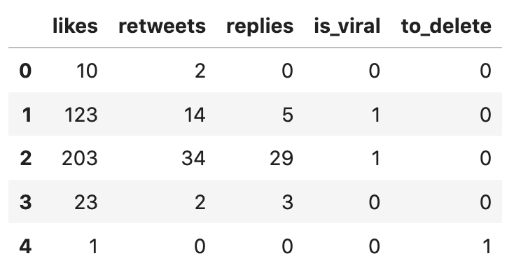
import pandas as pd
import numpy as np
from sklearn.model_selection import train_test_split
from sklearn.ensemble import RandomForestClassifier
from sklearn.metrics import accuracy_score
df = pd.read_csv("tweets-viral-delete.csv")
df.head()

Here's the current dataframe:

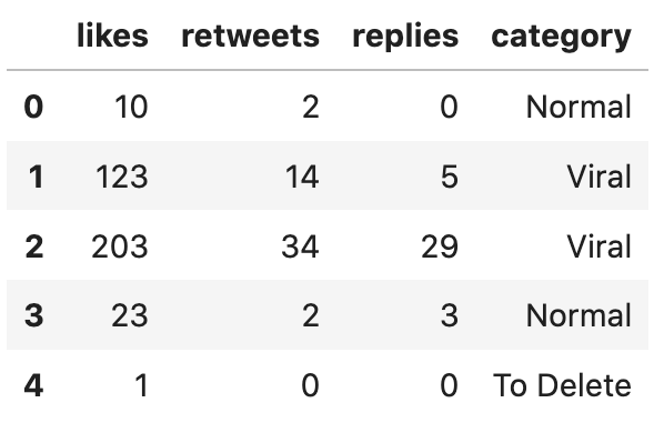
Now, let's apply a few functions from the pandas library. We also define our own function categorize() with an if-statement.

def categorize(row):
    if row['is_viral'] == 1:
        return 'Viral'
    elif row['to_delete'] == 1:
        return 'To Delete'
    else:
        return 'Normal'
 
 
df['category'] = df.apply(categorize, axis=1)
df = df.drop('is_viral', axis=1)
df = df.drop('to_delete', axis=1)
df.head()

As you can see, we created a new column df['category'] and then dropped two old columns (the axis=1 parameter means dropping a column and not a row).

The new updated dataframe:

Let's also see how many of each category we have:

df['category'].value_counts()

# Result:
category
Normal       58
Viral        26
To Delete    16
Name: count, dtype: int64

Model: Build, Train, Predict, Evaluate

Now that we have the data categorized, we can apply the same script from the previous lesson. The only difference will be the result of y, ' which will be one of the text values.

x = df.iloc[:,:-1].values
y = df.iloc[:,-1].values
x_train, x_test, y_train, y_test = train_test_split(x, y, test_size=0.2, random_state=0)
 
clf = RandomForestClassifier()
clf.fit(x_train, y_train)
y_pred = clf.predict(x_test)
y_pred

# Result:
array(['Normal', 'Normal', 'Viral', 'Normal', 'Normal', 'Normal',
       'Normal', 'To Delete', 'Normal', 'Normal', 'Normal', 'To Delete',
       'Normal', 'Normal', 'Normal', 'Viral', 'Normal', 'Viral', 'Normal',
       'Viral'], dtype=object)

The accuracy is... 95%!

accuracy_score(y_test, y_pred)
 
# Result: 0.95

Let's see which one the model predicted incorrectly:

df_compare = pd.DataFrame(
    data={
        'likes': x_test[:,0],
        'retweets': x_test[:,1],
        'replies': x_test[:,2],
        'predicted_value': y_pred,
        'real_value': y_test
    },
    columns=['likes', 'retweets', 'replies', 'predicted_value', 'real_value'])
df_compare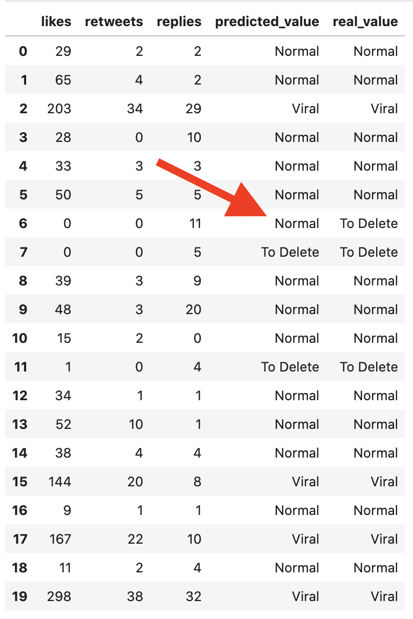

Based on the training data, the model decided that 11 replies is enough for a tweet to "survive", but this is a case of 0 likes and 0 retweets is a more important factor, looking from the human judgment perspective.

So, as you can see, the whole logic works similarly for binary and multiple classification, at least with the Random Forest algorithm.

Again, this dataset is close to "ideal", with a clear vision of which tweets should be viral or deleted, so the accuracy of 95% is logical.

Full Code

You can check out the Jupyter Notebook for this example here.

Or, if you prefer IDE like PyCharm, copy-paste this code there:

import pandas as pd
import numpy as np
from sklearn.model_selection import train_test_split
from sklearn.ensemble import RandomForestClassifier
from sklearn.metrics import accuracy_score
df = pd.read_csv("tweets-viral-delete.csv")
print(df.head())
 
 
def categorize(row):
    if row['is_viral'] == 1:
        return 'Viral'
    elif row['to_delete'] == 1:
        return 'To Delete'
    else:
        return 'Normal'
 
 
df['category'] = df.apply(categorize, axis=1)
df = df.drop('is_viral', axis=1)
df = df.drop('to_delete', axis=1)
print(df.head())
 
print(df['category'].value_counts())
 
x = df.iloc[:,:-1].values
y = df.iloc[:,-1].values
x_train, x_test, y_train, y_test = train_test_split(x, y, test_size=0.2, random_state=0)
 
clf = RandomForestClassifier()
clf.fit(x_train, y_train)
y_pred = clf.predict(x_test)
print(y_pred)
 
print(accuracy_score(y_test, y_pred))
 
df_compare = pd.DataFrame(
    data={
        'likes': x_test[:,0],
        'retweets': x_test[:,1],
        'replies': x_test[:,2],
        'predicted_value': y_pred,
        'real_value': y_test
    },
    columns=['likes', 'retweets', 'replies', 'predicted_value', 'real_value'])
print(df_compare)

In the following lessons, we will look at text classification, which is more common in real-life scenarios.

But before doing that, let me (finally) explain how Random Forest actually works, in the next lesson.